Dear all! As we promised last time, please, meet these rather useful (we hope) notes on How to Evaluate Face Recognition Software, on behalf of our software engineering and biometrics research team.
Preface
Neural network face recognition has recently gotten a lot of attention from business and government interests, as it provides a plethora of obvious advantages. We at NtechLab constantly get inquiries, testing requests, and pilot projects based on our latest technology and recognition techniques.
Benchmarking an algorithm of face recognition software can be a tricky process having many potential pitfalls. We’ve found out that sometimes people have difficulty translating their goals and ideas into software requirements. As a result, inappropriate tools can be chosen for the task at hand, and potential benefits get lost.
We decided to publish this memo in order to help people get more comfortable around a lot of the language and raw numbers surrounding methods and techniques of accurate face recognition technology. Our goal is to explain the core concepts of the field in a simple and concise way and to build a bridge between business and technical mindsets that ultimately results in better data-driven decisions and proper understanding of face recognition software in real-world use-cases.
Face recognition technology tasks
The term «face recognition» might include a number of disjointed tasks, such as detecting human faces in an image or video stream, gender recognition, age estimation, and identifying one person across multiple images and verifying that the two images belong to the same person. In this latest note, we will focus on the latter two, referring to these tasks as identification and verification, respectively.
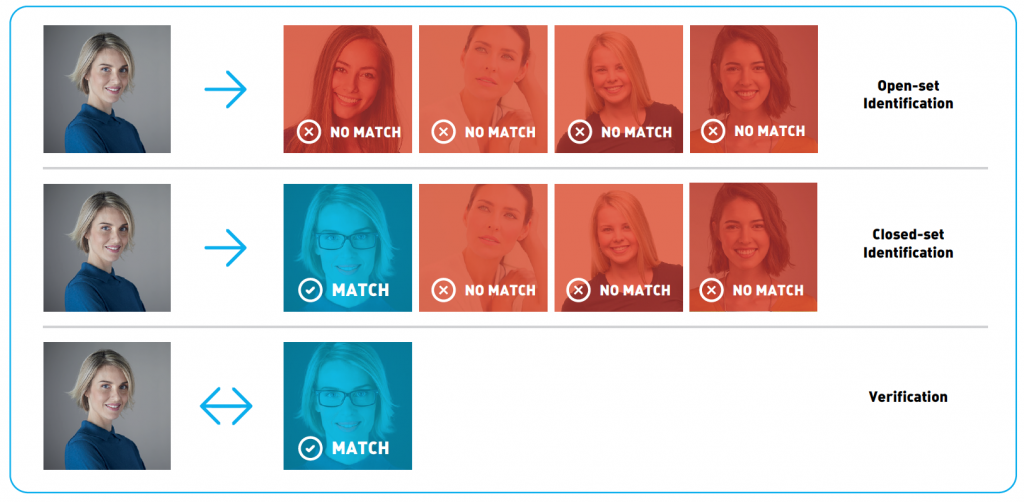
One common way to address these problems is to extract specially crafted descriptors, often called feature vectors, from the face image. Identification can then be reduced to a so-called «nearest neighbor» search, and verification can be performed by some simple decision rules. In combination, these two can identify a person in an image or determine if that person is absent from the prepared set of images. Such a procedure is called «open-set identification» (Figure 1).
In order to measure the similarity between the two faces, one can use a distance function in the feature vector space. The Euclidean and cosine distances are two of the most commonly used functions, but many other approaches of varying complexity exist as well. The specific distance function is usually shipped as part of the face recognition software. The approaches to identification and verification tasks differ in terms of the expected result, and different performance metrics are used in order to evaluate the facial recognition algorithms. The details of the metrics and their practical meaning are present in further sections. Apart from the metrics, an appropriately labeled dataset must also be available.
Evaluation
Dataset
Nearly all modern face recognition methods make heavy use of machine learning (or deep learning) throughout its processes. These systems are trained on large datasets of labeled images, and the quality and nature of the dataset have a great influence on the algorithm’s performance. The better the source data, the better matches the software can make.
A natural way to research and quantitatively measure whether different algorithms for face recognition meet one’s expectations and how accurate they are is to test it on a hold-out dataset. It’s crucial to choose an appropriate dataset for testing. Ideally, you’d have a separate dataset for testing purposes, which should match the use-case scenario as close as possible.
That means trying to replicate the camera type, filming conditions, age, gender of the people appearing in the test datasets. Adopting the dataset more similar to the data that the software will actually be processing makes the results of the testing more reliable. It’s usually a good idea to invest time and money into collecting and labeling of the dataset closest to the business problem, but in case this is not possible, as one has to resort to using public datasets of people’s faces.
Common public face recognition benchmarks include LFW and MegaFace. The LFW dataset contains only 6,000 pairs of faces, which makes it unsuitable for many practical applications: you can’t use it to measure reasonably low error rates, for instance, which we will show in further sections. The MegaFace dataset contains far more images and is appropriate for testing face recognition applications at scale. Both the training and testing parts of this dataset are freely available, so one must take special care while using it for testing, for the reasons discussed in the next section.
Another option is to use the test results provided by a trusted third party. These tests are performed by skilled personnel on private datasets, so their quality can be depended upon. One example is the NIST Face Recognition Vendor Test (FRVT) Ongoing (a downside of this approach is that the tester’s dataset might not match your usage scenario closely enough.)
Overfitting
As we have said, machine learning and computer vision are the main components of modern face detection techniques and recognition methods. One common (and sad) phenomenon associated with machine learning is called «overfitting,» which is what happens when the software performs well on the data it was trained on but loses its advantages on a new set of data.
To illustrate this concept with a concrete example: suppose a customer wants a system that opens a door only for certain people, verified by their faces. For this purpose, he collects photographs of the people to have access, then trains an algorithm to distinguish these people from others. Once field testing goes well and the system is deployed into production, the savings from securely automating that access point can be invested into other business purposes.
All of a sudden, the system fails to grant access to new employees. The software learned to recognize the old employees, but no one tested it on new data. This is an exaggerated example of overfitting, but it still serves to illustrate the concept.
The methodology of overfitting detection is not so simple; consider the cases where face recognition software is trained on a dataset consisting mostly of people of one ethnicity. When this biometrics software is deployed in a multinational region, the system’s facial recognition accuracy will most probably degrade. What is common among these examples is the overestimation of the software’s capabilities due to improper testing. The key performance flaw lies in the data it was trained on, and not the data that it is going to encounter in the real world.
So how does one avoid these situations? The key takeaway: don’t use a software training dataset for testing purposes. The safest and fastest way to do the research is to have a reserved testing dataset that wasn’t seen by the software vendor. If you are going to test the public dataset, make sure the vendor didn’t use it during training and calibration. Ask them which data sources they used for training, then choose a dataset that doesn’t appear on the ranking list. Have a look at the dataset prior to the testing, and consider its similarity to the data the software is going to encounter at the production stage.
Metrics
Once the test dataset has been chosen, one should consider the choice of an appropriate testing metric. A metric is a handy function that uses software outputs (either identification or verification) to produce a single number used as an overall measure of the system’s performance on the given dataset. A single number makes it easier for the decision-maker to quantitatively compare the vendors and concisely presents the test results. In this section, we will discuss the metrics commonly used in face recognition, and their business significance.
Verification
Face verification can be understood as a binary decision: yes, the two images are of the same person, or no, the images do not match. In order to understand the metrics used for verification, it is useful to spend some time studying this case’s error sources.
Given the two «accept» or «reject» predictions of the software and two «accept» or «reject» true outcomes, it is easy to see that there are 4 possible outcomes in total:

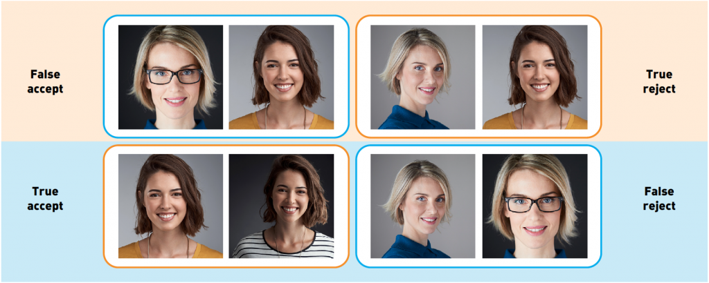
Of these outcomes, two are correct and the other two are known under different names. A Type I error is known as «false accept,» «false positive,» and «false match,» while Type II is called «false reject,» «false negative,» and «false non-match.»
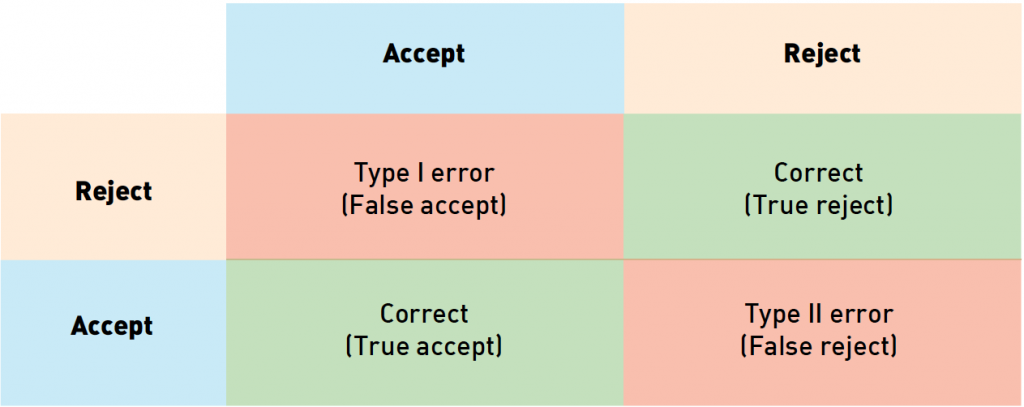
When we add up the number of errors in the dataset and divide by the dataset size, we get a false accept rate (FAR) and a false reject rate (FRR). In a security scenario, «false positive» corresponds to letting a wrong person in, while «false negative» means you deny access to an authorized person. These errors are distinguished because each one has different business costs associated with them. Going back to the security example, a false negative error might require a security person to double-check the employee’s ID Accidentally letting a malicious intruder in might lead to far worse consequences.
Given that the costs of errors are different across applications and use-cases, face recognition software vendors often provide the fastest way to tune the algorithm to minimize certain types of errors. In order to achieve this, the algorithm might output a continuous value reflecting its confidence, as opposed to a binary yes/no decision. The user can establish a threshold in order to minimize certain error rates. This value might be called confidence, similarity, or certainty, but we’ll refer to it as confidence throughout this document.
To illustrate this concept: consider a small dataset of 3 images. Image 1 and 2 are of the same person, while image 3 is of someone else. Let the software output the following confidence values for each of the 3 possible pairs:

We have picked values such that it’s impossible to get all the pairs correctly with any threshold. Choosing any threshold below 0.6 would result in two false accepts (one for pairs 2−3, one for pairs 1−3). We can clearly do better than that.
Choosing anything between 0.6 and 0.85 will rule out the 1−3 pair as a true reject, keeping 1−2 as true accept and 2−3 as false accept. The range of 0.85−0.9 will switch 1−2 to a false reject. Thresholds above 0.9 will result in two true rejects (1−3 and 2−3) and one false reject (1−2). Therefore the two most appealing threshold values are 0.6−0.85, which results in one false accept (2−3) and a threshold above 0.9 (which results in a false reject of the 1−2 pair). This example should demonstrate how a customer can measure his risks depending on the cost of each error, and minimize them by choosing an appropriate threshold. The ranges for the thresholds are a bit loose for this particular case because the dataset is so small and the certainty values are picked this way. For bigger, real-world datasets, one can find much tighter boundaries on the threshold for the accept/reject rates of interest. Vendors often provide some default values for the thresholds at some fixed FARs, and these values are precalculated in a similar way as we have described above.
One of the advantages in the FAR of interest decrease is the increase in the number of positive image pairs required to accurately measure the threshold. One needs at least 1,000 pairs to measure FAR=0.001, and FAR=10−6 would require more than 1 million pairs. Collecting a dataset of this size is challenging, so customers interested in very low FARs might consider public benchmarks like the NIST Face Recognition Vendor Test (FRVT) or MegaFace. Remember to treat these datasets with care, since the training and test datasets are freely available and overfitting (see the corresponding section) is likely to occur.
ROC curves
Error types differ in terms of costs, and the customer has the means to control the tradeoffs between error types. In order to do so, one has to study a range of threshold values. This can be tiresome. One of the handy mechanisms involved in visualization of an algorithm’s performance across a number of different FAR values is called a receiver operating characteristic (ROC) curve.
Let’s see how one can calculate and analyze an ROC curve. The confidence values (and therefore, the thresholds) can take a number of values in a fixed interval. In other words, they are bounded from above and below; let’s assume that this interval is 0−1. Now one can perform a bunch of evaluations with different threshold values, starting at 0 and increasing the threshold by some fixed amount until it’s equal to 1. For each threshold value, we record the FAR and true accept rate (TAR) (one could also use for example FAR and FRR). We then plot each point so that the FARs correspond to the X coordinates and the TARs correspond to the Y coordinates.
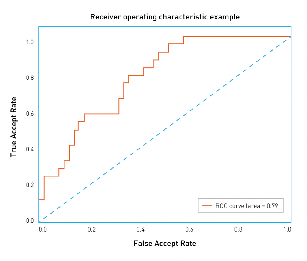
It’s easy to see that the first point will have coordinates 1 and 1. With a threshold of 0, we accept all pairs and do not reject any pairs. Similarly, the last point will be 0 and 0. With a threshold of 1, we accept no pairs and reject all pairs. With these two points fixed, the curve is usually convex upwards. One can see that the worst curve is somewhere on the diagonal of the plot and corresponds to random guessing. On the other hand, the best possible curve forms a triangle with points (0,0), (0,1), and (1,1). This is rarely seen in practice on sizable datasets.
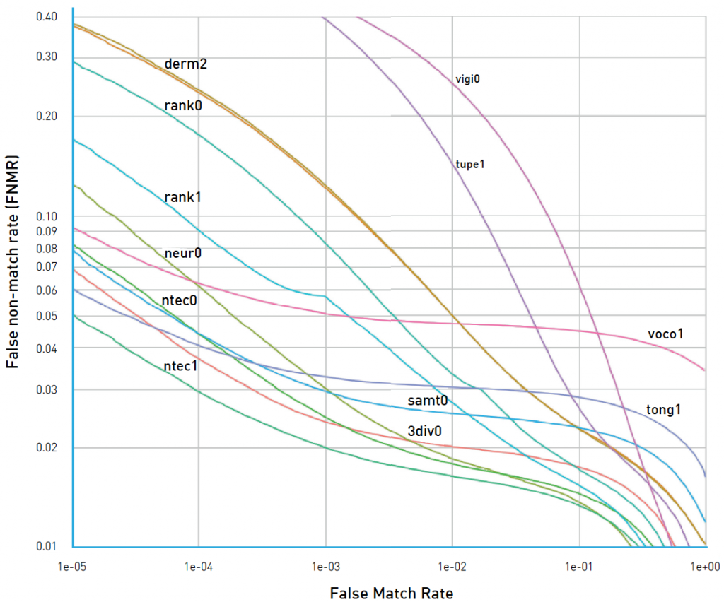
Fig 4. An ROC-like curve from NIST Face Recognition Vendor Test ranking
One can also calculate and plot ROC-like curves with different metrics/errors on the axis. For instance, consider Figure 4. Here the organizers of the NIST FRVT chose to plot the False non-match rate (FRR) as a function of false match rate (FAR). In this case, the best performing curves are lower and closer to the left, which corresponds to lower FRRs and FARs. Such variations should not confuse the reader, who is familiar with error types, just take some time to read and comprehend the axis names.
This plot makes it easy to see how well the algorithm performs at a chosen FAR; one just has to find a matching point on the curve and a corresponding TAR value. There’s also a way to express the «goodness» of the ROC curve in one number; just calculate the area under the curve with the best value being 1, and a random guess corresponding to 0.5. This number is called ROC AUC (Area Under Curve). One should note though that ROC AUC makes an implicit assumption that different error types have the same cost, which is not true in practical applications. One should rather study the shape of the curve, paying special attention to the FAR values that match business needs.
Identification
Another task involved in the recognition methodology is the identification, which essentially tries to find a specific person among a number of facial images. The results are sorted by confidence value, with the items the algorithm is most sure about appearing at the top. Depending on whether or not it is known that the target person is present in the set, identification can be divided into two subcategories: closed-set identification (the person is in the set) and open-set identification (the person may or may not be in the set).
A reliable, interpretable metric for measuring closed-set identification is accuracy. In a nutshell, accuracy measures the average number of times the target person shows up among the search results.
Let’s see how this works in practical terms. As usual, we start by stating the business requirements. Imagine we have a web page where up to 10 search results can appear. We should, therefore, measure the number of times the correct person is found among the top ten search results. This is called Top-N accuracy, and in this particular case, N equals 10.
For each research instance, we set aside a target image of a particular person to find and the gallery set we are going to search through, containing at least one other image of the same person. We then retrieve the top ten search results and check whether the target person is among the results. In order to get the accuracy value, one adds up the trials where the person was found, then divides by the total number of trials.

Open-set identification consists of retrieving the image most likely to be the target person, then deciding whether or not it is indeed this person based on the confidence value. Open-set identification can be seen as a superposition of closed-set identification and verification, and all the discussion on evaluating verification tasks applies here. It’s also clear that one can perform open-set identification by verifying the target image with every other image in the search set. The reason people use closed-set identification here is efficiency; some face recognition software ships with the fastest search algorithms capable of going through millions of vectors of features in milliseconds. Doing this many distinct verifications will take much more time.
Case studies
In order to illustrate the above topics, let’s have a look at a couple of examples of how one might evaluate human face recognition software for a practical use-case.
Retail shop
Consider a medium-sized retail shop that wants to improve its loyalty program and get rid of shoplifters with the benefits of biometrics systems. The two tasks are nearly the same, as far as accurate face recognition is concerned. The goal of the project is early detection and recognition of the loyal customer or shoplifter, ideally at the shop entrance, by comparing face images and reporting to a salesperson or security as needed, which will also help to improve the service.
Suppose that there are 100 people in the loyal customer list. This can be seen as an example of open-set identification. After considering the costs, the marketing department decides that it’s acceptable to mismatch one visitor as a loyal customer daily. Assuming that the shop sees a daily average of 1,000 visitors, each has to be matched against a list of 100 loyal customers. The necessary FAR can be estimated as 1 / (1000 * 100) = 10−5, which corresponds to about one customer per day recognized as loyal by mistake.
Once the error rates are set, one should consider choosing a proper dataset for testing. One good course of action might be to install a camera in the desired location (face recognition vendors can help with recommending devices and locations). By matching the transactions from the loyalty cardholder with the camera images and filtering the results by hand, the shop employees can build positive pairs dataset. It’s also a good idea to add a bunch of random visitor images (one image per person) This number of images should be roughly equal to the daily average number of visitors to the shop. By combining the loyal customer images with random visitor images, one can build a test dataset of both positive and negative pairs.
One thousand positive pairs should be enough for a desirable detection rate. The negative pairs can be formed by combining different loyal customers and random visitors. It’s easy to get as many as 100,000 negative pairs this way.
The next step is to run (or ask the vendor to run) the face recognition software and to obtain the confidence scores between all the image pairs in the dataset. Once this is ready, you can plot an ROC curve to make sure that the number of correctly recognized loyal customers (TAR) at FAR=10−5 meets your business goals.
Airport e-gate
Modern airports serve tens of millions of passengers annually, which means some 300,000 people pass their ID controls every day. Automating this access control might save a lot of money for the airport. (On the other hand, the cost of letting a trespasser in is also very high, and the airport management would like to keep the risk of this outcome as low as possible.) An FAR of 10^-7 might seem reasonable in this case. This will result in allowing 10 trespassers on average per year. Assuming FRR=0.1 at this point, which corresponds to NtechLab’s results on the visa images dataset at this FAR, this will result in a 10x decrease in manual ID-checking.
This dictates a need for a dataset of 10−7 images. Unfortunately, collecting and labeling a dataset of this size is costly and may give rise to privacy issues. This might make such a project too much of a long-term investment for some organizations. In these cases, it makes sense to cooperate with law enforcement or other government agencies in order to obtain a dataset for testing. You might study the NIST FRVT report, which has visa images as one of its testing datasets. Airport management should choose a vendor based on the evaluation of this dataset and the passenger flow in the given airport.
Targeted Email Marketing
So far we’ve seen examples where low FARs were of primary concern, but there’s more to the story. Imagine an advertisement in a shopping mall that’s been equipped with a video camera. The mall has a loyalty program and would like to recognize customers who stopped by the advertisement, sending them targeted emails with deals and personalized offers based on what caught their eye.
Let’s say the cost of maintaining this system is $ 10 per day, and 1,000 customers stop by each day. The marketing department estimates that one such targeted email will net $ 0.0105. We would like to hit as many target customers as possible without bothering the others too much. In order for the advertisement to pay off, the target accuracy should be equal to the cost of the stand divided by the multiple of passersby and email value. For our example, accuracy = 10 / (1000 * 0.0105) = 95%. One can obtain the dataset similar to the «Retail shop» example, measure the accuracy as described in the «Identification» section, and based upon the result, decide whether the tested software will be able to meet the business goals.
Practical considerations
Video support
Throughout this piece, we’ve been discussing the processing of the facial images without focusing on the video stream. Video can be seen as a series of successive still images, so the metrics and testing approaches that work for still images also work for video. It should still be noted that processing video streams is much more computationally expensive and puts additional constraints on all components of the face recognition mechanisms. Measure the algorithm’s execution time while dealing with video. Such timing is straightforward to do and is not covered in this document.
Common mistakes
In this section, we would like to list common issues that arise during face recognition software testing and give guidelines to improve on them.
TESTING ON AN INSUFFICIENT DATASET
One should be very careful when choosing an appropriate dataset for the evaluation of the benefits of face recognition systems. One of the key issues to consider is the dataset size. The size of a dataset should be chosen with the business goals and specific FAR/TAR values involved. Playing around with tiny datasets of several people collected in the office might give a sense of how to use the software benchmark execution time, or try out tricky, specific use-cases. But small datasets don’t help in estimating the algorithm’s overall accuracy. Please use sizeable datasets for evaluating accuracy.
USING ONLY ONE THRESHOLD FOR TESTING
Sometimes people test face recognition software at one fixed threshold value (often the default) and only consider one type of error. This is not the way to go since default threshold values vary between vendors using different FARs or TARs. One must always consider both metrics for a set threshold value.
COMPARING RESULTS ON DIFFERENT DATASETS
Datasets differ widely in terms of size, quality and complexity, so human face recognition software results are not comparable between datasets. It’s easy to reject an otherwise superior algorithm just because it was tested on a more challenging dataset than its competitors.
RELYING ON A SINGLE DATASET
One should try to test the algorithm on several datasets. It might be a bad idea to use a single public dataset for evaluation since you can’t make sure that the face recognition software vendor didn’t use this dataset for algorithm training or tuning. If that’s the case, the tests will likely overestimate the algorithm’s accuracy. Luckily, this situation can be avoided by comparing performance across several different datasets.
Conclusion
In this memo, we have briefly discussed the key components and mechanisms of evaluating a face recognition algorithm: datasets, tasks, corresponding metrics, and common scenarios.
Of course, there’s more to the story, and numerous one-off cases should be handled separately (the NtechLab team would be happy to help with those). Still, we believe that after reading these notes the reader should have a solid understanding of the key concepts, be able to plan the software testing, interpret the results meaningfully, and measure the pros and cons of different algorithms as they seek to reach various business goals.
